


Causal Inference — Double Machine Learning
Introduction

Introduction
Ever heard of the term Double Machine Learning (Double ML) and wondered what it is? Double ML is a powerful technique for causal inference, offering significant advantages over traditional methods like Linear Regression. In this article, we will explore the concept of the causal inference using observed data, discuss the limitations of Linear Regression, and demonstrate how Double ML can provide more accurate and robust causal estimates. Through a practical example, we will illustrate the steps involved in implementing Double ML and interpreting its results.
Business problem
Imagine that you are a data scientist working as part of a marketing science team. Your marketing team wants you to measure the causal impact of advertising spend on sales. While Randomized Controlled Trials (RCTs) are the gold standard for causal inference, they are often impractical or infeasible in real-world marketing scenarios due to logistical and ethical constraints.
However, estimating the causal impact from historical data is more challenging due to confounders which affect both treatment and outcome. For instance, seasonal fluctuations and long-term trends can confound the relationship between advertising and sales. Without accounting for these confounders, causal estimates can be biased, hindering accurate measurement of the impact of marketing efforts. We are going to learn how we can overcome these challenges using causal inference techniques like Controlled Linear Regression and Double ML.
Note — This article will delve into the methodologies employed, their associated benefits and drawbacks, and the resulting outcomes. For those seeking a deeper dive into the underlying code, the complete repository is available on GitHub.
Data Generating Process
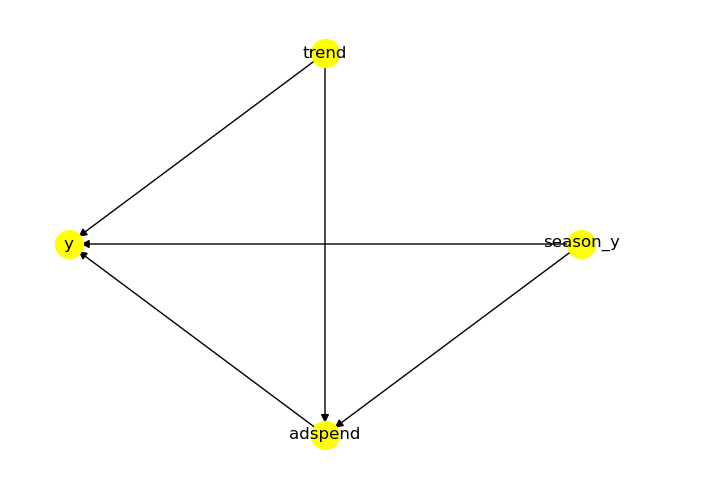
For our hands-on example, we are going to generate simulated data. Usually, marketing acts as a multiplier of sales and has both delayed and diminishing returns. In order to capture this relationship accurately, we would have to build a non-linear model. To keep things simple, let’s assume a linear, additive relationship between our outcome (sales), treatment (advertising spend) and confounders (seasonality, trend). Figure 1 below shows the causal diagram for this simplified data generation process.
Note —Also, in practice, there could be many other predictors or confounders like pricing, distribution, promotion, etc. affecting sales and advertising spend.
Here is the code used to generate the simulated data
# Set random seed for reproducibility
np.random.seed(42)

# Create a time series index
date_range = pd.date_range(start='2020-01-01', end='2023-12-31', freq='W-MON')

# Create a dataframe
df = pd.DataFrame({'week': date_range})

# Create trend component
df['trend'] = np.linspace(100, 300, len(date_range))

# Add seasonal component
df['seasonality'] = 50 * np.sin(2 * np.pi * df.week.dt.isocalendar().week / 52)

df['baseline_sales'] =  df['trend'] + df['seasonality']

# Add media driven sales
df['media_incremental_sales'] = 0.3 * df['baseline_sales']
df['adspend'] = df['media_incremental_sales'] /2

# Calculate total sales
df['sales'] = df['baseline_sales']  + 2 * df['adspend'] + np.random.normal(loc=0, scale=15, size=len(date_range))
Exploratory Data Analysis
Let’s visualize the components of simulated sales data and understand the ground truth.


Observations
We have a linear trend
Yearly seasonality follows a sine curve
Media incremental is correlated with trend and seasonality
For every $1.00 increase in ad spend, we expect to see a $2.00 increase in sales
Note — In real life, we won’t know the ground truth. Typically, we try to narrow down our belief of ground truth using multiple different approaches like A/B testing, MMM, causal inference, MTA, etc.
Prepare Modeling Data
From here on, we are going to act as if we don’t know anything about the data generating process and try to recover the causal effect of advertising spend on sales. Our dataset would have total sales and advertising spend.
First, let’s try to recover the trend and seasonality components of sales using Prophet. If you are new to using Prophet, here is a good tutorial to understand all the functionalities.
df_model = pd.DataFrame()
df_model['ds'] = df['week']
df_model['y'] = df['sales']
df_model['adspend'] = df['adspend']

prophet = Prophet(yearly_seasonality=True)
prophet.fit(df_model)
prophet_predict = prophet.predict(df_model)
with warnings.catch_warnings():
    warnings.simplefilter("ignore", FutureWarning)
    plot = prophet.plot_components(prophet_predict, figsize = (12, 8))

prophet_columns = [col for col in prophet_predict.columns if not col.endswith(("upper", "lower"))]

df_model["trend"] = prophet_predict["trend"]
df_model["season_y"] = prophet_predict["yearly"]
Now, let’s check the correlation between all the variables.

Observations
As expected, adspend is correlated with sales (y) as well as trend and seasonality
Trend and seasonality are as well correlated with sales
This correlation matrix confirms our causal diagram. Trend and Seasonality are confounding impact of adspend on sales.
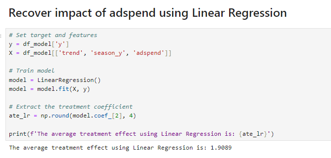
Modeling — Controlled Linear Regression
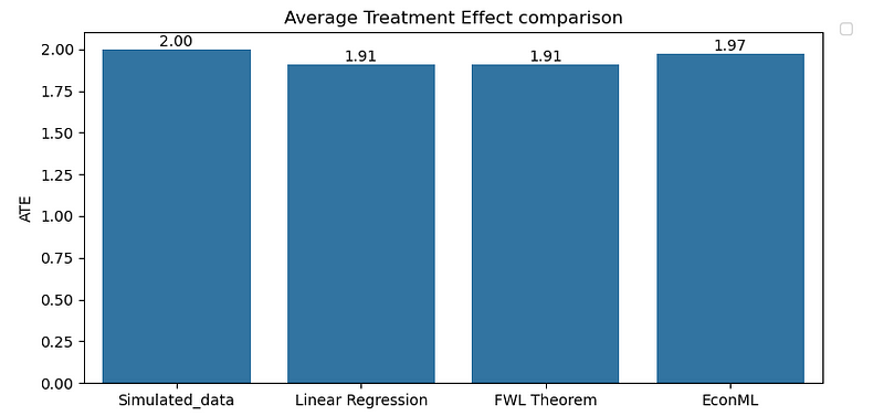
This is our baseline model. We are going to regress sales on advertising spend while controlling for confounders like trend and seasonality. Causal effect, measured as Average Treatment Effect (ATE), after conditioning on confounders is 1.9089. This is pretty close to our ground truth.
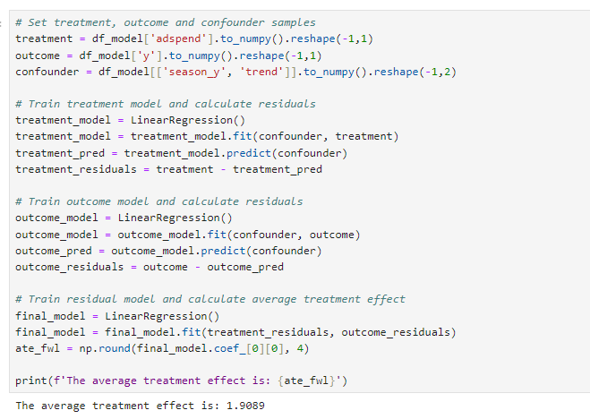
Modeling — Frisch-Waugh-Lovell (FWL) theorem
FLM theorem provides a foundational framework for various de-biasing techniques, including Double Machine Learning. Essentially, it’s a method for making observational data appear as if it were generated from a randomized experiment. The theorem states that a multivariate linear regression model can be estimated either in a single step or in three separate stages. This concept has been extended to more general contexts, one of which is Double ML. Figure 7 below illustrates the three-step process outlined in the FWL theorem.

Let’s apply this theorem to our hands-on example and take a look at the results. As we notice in Figure 8, we end up with exactly same ATE of 1.9089 as linear regression.
Modeling — Double ML
Controlled Linear Regression performed really well in our simplified use case. However, it really struggles to capture the causal effect when we have high dimensional features or when relationships are non-linear. Also, Linear Regression doesn’t help us measure Conditional Average Treatment Effect (CATE).
Double ML addresses all of the above challenges of Linear Regression. Double ML employs a three stage process similar to FWL theorem to measure causal estimate. The key advantage is that Double ML doesn’t rely on strong parametric assumptions like linear regression, making it adaptable to a wide range of real-world data scenarios.
Here are a couple of example scenarios
Non linear relationship between continuous treatment and continuous outcome — Double ML can utilize other ensemble techniques like Random Forest to capture the non-linear relationships across all 3 steps.
Non linear relationship between discrete treatment and continuous outcome — Double ML can utilize LogisticRegression() for debiasing step to model the propensity score (probability of receiving the treatment), RandomForestRegressor() for denoising step and bring them together in the 3rd model where propensity score weights are used to adjust for the selection bias.
Measuring CATE : Double ML is particularly well-suited for estimating CATEs, which allow you to examine how treatment effect across across different subgroups of the population. Conversely, it can also help identify subgroups of population that respond differently to the treatment.
Coming back to our example, let’s try implementing Double ML using DoWhy and EconML package. DoWhy offers a structured 4-step framework for causal inference:
Draw DAG: Visualize the relationships between variables and identify potential confounders.
Identify Estimand: Specify the causal question and the target estimand (e.g., Average Treatment Effect).
Estimate: Employ DML or other appropriate methods to estimate the causal effect.
Validate: Assess the robustness of the results to potential unmeasured confounders.
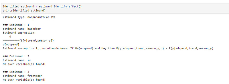
EconML provides a collection of methods for causal inference, including Double ML. By combining DoWhy’s framework with EconML’s implementations, we can efficiently conduct causal analyses and leverage the best of both worlds. Figure 9 below shows that DoWhy identified a backdoor estimand for our problem and recommends conditioning on trend and seasonality to measure causal impact of adspend on sales.
Next, let’s estimate the adspend causal impact on sales. Figure 10 shows that we are calling LinearDML() from within DoWhy’s estimate_effect(). Causal effect measured using this approach is 1.9709 which is pretty close to our ground truth again.

Finally, we can also use DoWhy to run a placebo treatment to validate our results. Figure 11 shows that if we replace actual treatment with a placebo, ATE drops from 1.97 to ~0. This clearly proves that the effect measured is valid.

Conclusion
In our simplified example, we observed similar results from Controlled Linear Regression, FWL Theorem, and Double ML. While this provides a foundational understanding, real-world scenarios often present greater complexities, such as high-dimensional data, non-linear relationships, and unmeasured confounders.
Double Machine Learning’s ability to handle these challenges underscores its versatility and effectiveness in causal inference. As research in this field continues to evolve, we can expect even more advanced techniques and applications to emerge.
I look forward to exploring these developments further and sharing my insights in future articles.
References
“Causal Inference in Python” by Matheus Facure (O’Reilly). Copyright 2023 Matheus Facure Alves, 978–1–098–14025–0